We trust you have been following along and created your first report from SQL using the basic tools build into excel. Now that you have the data, it is time to build intelligence into your business data. Some people call this BI and want to make it fancy and complicated, but it really is not.
To build intelligence into your business data, you just have to summarize and graph your data. You see, most of your audience will have a zillion things going on and your report is performing in the “short attention span theater”. You need to get your point across, and you need to do it quickly. One page summaries and graphs are key and pivot tables are a quick and easy tool. Once built, you can easily update (or refresh) your results as your data changes… easily keeping your report up to date!
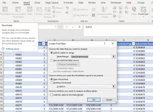
On your excel report, you need to be someplace within your results from SQL. From there, in your ribbon bar, click “Insert” then “Pivot Table and a window of options will appear. The best way to start is to take all the defaults and let Excel create a new worksheet. If this is acceptable, just click “OK” and your new worksheet will appear.
When we initially created the data table, we stressed giving a meaningful name. The same applies to a Pivot Table. The default name will be “PivotTable1” which might be ok to memorialize this as your first Pivot Table… or rename it “SalesOrderSummary”.
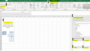
After creating the pivot table, you will see a blank slate, with several important areas. Take a moment to look here:
 Pivot Table Name
- Additions to Ribbon Bar. Note the new boxes “Analyze” and “Design”
- Pivot Table data area. This is where data will display once added to the summary
- Pivot table fields. This is the list of all the fields you included in your SQL query. Initially, each are “unselected”.
- Filters. Here you will place fields you want to use to allow a user to narrow down data they are displaying. You have other ways to do the filters, but this makes for easy usage.
- Rows is for the items where the results will display down.
- Columns is fields were the results will display across
- Fields that will be the numeric data to be summarized or counted.
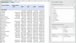
Now that you know the key points in a Pivot Table, we are finally… finally… at the point to Build Intelligence into your Business Data. Using basic drag and drop techniques, pull data the various box. While you can do most anything you want here, for our example we recommend the following:
- Filter: TerritoryName
- Rows: StateProvidence
- Columns: Order Date. In early versions or Excel, all dates would be show across the top, possibly more than Excel can handle. In Excel 365, the Oder date is automatically summarized into three “groups” for Years, Quarters and Order Date. We discuss data grouping a bit later, either way just take the initial default.
- Values: Total Due, which will be summarized.
While certainly not a polished report, you were able to Build Intelligence into your Business Data with summary by state/providence for the four years of data available and no formulas were required!
Next we will discuss Pivot Table Cleanup.


